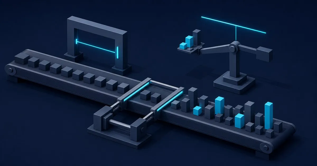
Concept Drift Detection Methods: DDM, ADWIN and More

Concept drift is the case where P(Y|X) changes: the relationship between your features and the label is no longer what the model learned. The features can look completely normal while the model is wrong, which is why input-distribution monitoring is structurally blind to it. A fraud model trained before a new attack pattern sees the same transaction amounts, the same merchant categories, the same device fingerprints. Only the answer changed.

That structural blindness is the whole difficulty. Data drift detection compares two distributions you both have. Concept drift detection needs the label, and the label is usually late. Every method below is an answer to some version of “how do I detect a change in P(Y|X) given what I actually have access to right now.”

If you are still separating the two failure modes, start with concept drift vs data drift explained, or with the full taxonomy in types of data drift. This piece assumes the distinction and goes into the detectors.

PSI vs CSI compares the stability checks on score distributions and individual characteristics. Neither calculation directly confirms a changed input-to-outcome relationship; keep the error or outcome stream separate.

The four shapes concept drift takes

The taxonomy comes from the 2014 concept-drift survey, and it matters because different detectors are tuned for different shapes.

Sudden. The relationship changes at a point in time. A policy change, a new competitor, a regulation taking effect, a fraud ring switching technique. Easiest to detect and the case every detector handles.

Gradual. Old and new concepts alternate, with the new one becoming more frequent. Customer preference shifts look like this. A detector tuned for sudden change will either miss it or fire late.

Incremental. The relationship moves continuously through intermediate states. Inflation shifting the meaning of a price feature is the standard example. No single change point exists to find.

Recurring. A previous concept returns. Seasonality, weekday and weekend behaviour, holiday shopping. The critical property is that this is not something to retrain away, and a detector without memory of past concepts will trigger a pointless retrain every cycle.

Real drift on a production model is usually a mixture, and the practical consequence is that a single detector with a single sensitivity setting will be wrong about part of it. Running a fast detector and a slow detector in parallel, and treating agreement as the signal, is a cheap fix.

Error-rate detectors: when labels arrive fast

If labels arrive within minutes or hours, the strongest signal is the model’s own error stream. These detectors watch a binary sequence of correct and incorrect predictions and flag when its rate changes more than sampling noise explains.

DDM (Drift Detection Method)

DDM tracks the online error rate p and its standard deviation s, and remembers the minimum of p + s seen so far. It raises a warning at p + s > p_min + 2·s_min and a drift alarm at p + s > p_min + 3·s_min, the classic three-sigma rule applied to a running error rate. Between warning and alarm, it buffers incoming examples so a new model can be trained on post-change data only.

DDM is fast, has almost no memory footprint, and handles sudden drift well. Its known weakness is gradual drift: a slow change never crosses the alarm threshold before the buffer overruns. EDDM addresses this by tracking the distance between errors rather than the error rate, which makes it more sensitive to slow degradation and correspondingly more prone to false alarms on noisy streams.

ADWIN (Adaptive Windowing)

ADWIN, introduced in the adaptive-windowing paper, keeps a variable-length window of recent values and repeatedly tests whether it can be cut into two sub-windows with statistically distinguishable means. When such a cut exists, the older sub-window is dropped and drift is reported. The window size is therefore not a hyperparameter, which is the whole point: it grows during stable periods and shrinks automatically when the stream changes.

The single tuning knob is a confidence parameter delta, with a rigorous false-positive bound attached to it. In practice ADWIN is the default recommendation for streaming settings, and it is the detector wired into most online-learning ensembles. It is also usable on any numeric stream, not just an error sequence, which means it can watch a feature mean or a calibration statistic.

from river import drift

detector = drift.ADWIN(delta=0.002)

for y_true, y_pred in label_stream:
    error = int(y_true != y_pred)
    detector.update(error)
    if detector.drift_detected:
        handle_drift(index=detector.n_detections)

Page-Hinkley

Page-Hinkley is a sequential change-point test that accumulates the deviation of each observation from the running mean and alarms when the cumulative sum departs from its own minimum by more than a threshold lambda. It is designed for a shift in the mean of a numeric signal, which makes it a better fit than DDM when the thing you are watching is a continuous quantity: mean absolute error on a regression model, average response latency, a calibration gap.

Two parameters control it. delta is the magnitude of change considered tolerable, and lambda is the alarm threshold. Both need fitting against a historical replay of your own signal. Copied defaults are the usual reason it either never fires or fires constantly.

KSWIN

KSWIN applies a two-sample Kolmogorov-Smirnov test between a sliding recent window and a reservoir sample of older data. It is distribution-based rather than error-based, so it detects a change in the shape of a stream rather than only its mean, and it inherits the KS test’s sensitivity to large sample sizes. On high-volume streams it will flag statistically real, practically meaningless differences unless the window is kept small.

Detector	Watches	Best for	Main weakness
DDM	Binary error rate	Sudden drift, low memory	Misses gradual drift
EDDM	Distance between errors	Gradual drift	Noisy on unstable streams
ADWIN	Any numeric stream	Sudden and gradual, no window tuning	Slower to compute
Page-Hinkley	Mean of a numeric signal	Regression error, latency	Two parameters need fitting
KSWIN	Distribution of a window	Shape changes, not just mean	Over-sensitive at high volume

When labels are late: estimating performance instead

Most production models are not in the fast-label regime. Chargebacks confirm in weeks, loan defaults in months, churn possibly never. Error-rate detectors have nothing to consume.

The approach that works is estimating performance from what you do have: the model’s own confidence scores plus the input distribution. NannyML’s Confidence-Based Performance Estimation reweights the model’s predicted probabilities by the observed covariate shift to produce an expected ROC AUC or F1 for the unlabelled period. Direct Loss Estimation does the analogous thing for regression by training a second model to predict the first model’s loss.

The load-bearing assumption is that the model stays calibrated. CBPE estimates what performance would be if the score-to-outcome mapping were unchanged, which means a divergence between estimated and eventual realised performance is itself the concept-drift signal. That is a genuinely useful property and also the trap: during actual concept drift the estimate is optimistic, precisely when you need it least. Treat estimated performance as an early-warning tripwire that gets confirmed against real labels when they land, never as a substitute for them.

The full set of tactics for the label-blind window, including proxy metrics and delayed backfill, is covered in monitoring models when ground truth is late or never arrives.

The label-free proxies, and their honest limits

Three signals move before labels do and are worth wiring up regardless.

Prediction drift. The output distribution shifting is consistent with concept drift, but also with input drift and with a correctly-functioning model responding to a genuinely changed world. It is a question, not an answer.

Calibration decay. If the reliability diagram bends away from the diagonal on the subset of data where labels have arrived, the score-to-probability mapping has moved. Partial labels are enough for this, which makes it usable well before full accuracy is computable. Metric selection here is covered in choosing monitoring metrics: PSI, KS, and calibration.

Segment divergence. Concept drift frequently starts inside one cohort: a geography, a channel, a customer tier. Aggregate accuracy can hold flat while one segment collapses. Breaking every signal down by two or three business-meaningful segments finds this, and it is the cheapest high-yield addition to most monitoring setups.

None of the three proves concept drift on its own. Together with a documented diagnostic order, they narrow it down fast, which is what the ML model monitoring framework step on actions is for.

Choosing a detector

The decision follows label latency more than anything else.

Labels in minutes to hours, streaming model. ADWIN on the error stream, DDM as a cheap second opinion. Retrain or adapt on agreement.
Labels in hours to days, batch model. Page-Hinkley or ADWIN on a daily error aggregate, plus prediction and calibration monitoring for earlier warning.
Labels in weeks to months. Estimated performance (CBPE or DLE) as the primary tripwire, input drift as the corroborating signal, realised performance as the eventual confirmation.
Labels never arrive. No concept-drift detector applies. You are monitoring inputs, outputs, and business KPIs, and accepting that the mechanism will be inferred rather than measured. Say so explicitly in the monitoring spec rather than pretending a drift chart covers it.

For recurring drift specifically, add a check before the retrain: if the detector fires on roughly the same calendar cadence it fired last year, the correct response is a seasonality-aware reference window, not a new model.

Practical failure modes

Retraining on the drift signal alone. A detector firing says the relationship changed. It does not say a retrain will help, and if the cause is an upstream pipeline break, retraining bakes the break into the model. Confirm the mechanism first; training-serving skew in particular masquerades as concept drift and is fixed in the feature pipeline, not the model.

Fitting the detector on a clean stream. Detector parameters tuned on synthetic or held-out data behave differently against production noise. Replay historical data through the detector and count how often it would have fired.

One detector for a mixture of drift shapes. Sudden and incremental drift do not share a sensitivity setting. Two detectors in parallel with agreement logic costs almost nothing.

Treating a warning as an alarm. DDM’s two-level design exists so that the warning level starts collecting post-change data while the alarm level triggers the response. Collapsing them into one threshold discards the buffered training window that makes recovery fast.

No memory of past concepts. Recurring drift on a detector without concept memory produces an endless retrain loop. Keeping previous model versions and their reference windows around lets you swap back rather than relearn.

For LLM-backed systems the detectors above mostly do not transfer, because there is no error stream and often no label at all; what does and does not carry over is covered in monitoring tabular models vs LLM systems and silent quality decay in production LLM apps.

Concept Drift Detection Methods: DDM, ADWIN and More

The four shapes concept drift takes